How should an overwhelming pool be sequenced so that every prefix holds the most net-new value per unit of effort? · vicente.md
vicente.md/2026-004 [cs.DS] · 17 Oct 2026
Preprint · not peer reviewed 9 pages
How should an overwhelming pool be sequenced so that every prefix holds the most net-new value per unit of effort?
Vicente González B.†
Engineer and Computational Neuroscience Researcher · Santiago, Chile
† correspondence · hi@vicente.md · no institutional funding, no competing interests
Abstract
Order inputs by residual density over prerequisite-closed bundles, and stop at the shadow price of attention. That rule answers a question many fields ask under different names. How should an overwhelming pool be sequenced so that every prefix holds the most net-new value per unit of effort? Residual density is an input’s value measured against what earlier inputs left unexplained, divided by its cost. Scoring bundles closed under prerequisites lets a foundation borrow the value of what it unlocks. The stop is the reader’s long-run rate of value per unit of effort, as information foraging theory predicts. Without prerequisites and with diminishing returns, each prefix holds at least 1 − 1/e of the optimum at its own cost; no efficient rule guarantees more. Synergy lowers that floor to 1 − e^(−γ), where γ is the submodularity ratio. Under prerequisites with additive value, Sidney’s bundle order keeps value-weighted waiting time within a factor of 2 of optimal. Coverage greedy, information gain, orthogonal least squares, aspect diversification and Sidney’s decomposition are all special cases. They differ only in how they represent the residual and the bundles.
The construct starts from a reading list. Facing a shelf of computational neuroscience books, the question was which to read first. The answer had to be a ranked list, sorted greedily by impact of knowledge per word, with compounding.
The list carried one hard requirement. Its first entries must hold the most fundamental knowledge, so that stopping early still leaves the most solid foundation. Every prefix of the list has to be a good list on its own.
Stated for learning, the question is how to select and sequence complex resources from an overwhelming pool. The goal is maximal net-new mastery per unit of effort, with no redundancy and no friction from missing foundations. Stated for systems, it is how to curate a stream of inputs for maximal net-new value per unit of cost.
Three words in the question carry its formal content. “Per word” is a cost, “compounding” is an interaction between inputs, and “every prefix” is an anytime objective.1
Question. How should an overwhelming pool be sequenced so that every prefix holds the most net-new value per unit of effort?
worst-case floor
exactly optimal
precedence factor
mean mastery
63.2%
93.4%
≤ 2×
12.1 of 28
of the optimum, at each prefix’s own cost
of chain prefixes, 80 random instances
Sidney order, weighted waiting time
closure density; 11.3 item by item
Four numbers from four parts of the argument: the guarantee under diminishing returns and what random coverage instances achieve in practice (Section 5), the guarantee under prerequisites (Section 6), and the seven-book example (Section 6).
Why a fixed score fails
Sorting by a fixed impact-per-word score fails because compounding has two signs. Each input interacts with what was already taken, and the two interactions pull in opposite directions.
Overlap. Two introductions teach much of the same material, so the second adds less than its score claims. A fixed score counts shared content twice.
Prerequisites. An advanced text pays off only after its foundations, so a fixed score credits it too early and the foundation too little. Missing foundations also raise cost: words absorb slower when the background is absent.
Overlap makes value submodular: an input adds less to a larger set. Prerequisites make value supermodular: an input adds more to a set that contains its foundations. A sound rule must therefore re-score after every pick, and must judge a foundation by what it unlocks.
The object: an ordering judged at every prefix
The answer is an ordering, and its quality is measured at every prefix. Four ingredients define it.
InputsV: books, chapters, papers, features or data sources.
Costc(e)>0: the words, hours or money that input e consumes.
Valuef(S): mastery of a weighted concept space after taking the set S, with f(∅)=0 and f never decreasing as S grows.
Prerequisites: a partial order on concepts; a concept counts as mastered only once its foundations are.2
For a budget B, the best set is OPT(B). Plotted against B, it traces the cost-value Pareto frontier.
OPT(B)=S⊆V,c(S)≤Bmaxf(S)
An ordering e1,e2,e3,… defines nested prefixes S0⊂S1⊂S2⊂⋯. The question asks that every prefix sit near the frontier at its own cost, all at once. That anytime demand is stronger than solving any single budget.
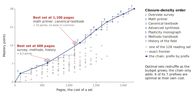
The exact frontier cannot meet it. Optimal sets at nearby budgets often share no members, so no single ordering passes through all of them. What the question really asks for is the best nested approximation of the frontier: the “greediest Pareto set”.
Figure 1. The exact frontier reshuffles; the chain nests. Every one of the 128 reading sets from the seven-book shelf of Section 6 is plotted by its pages and mastery points (grey dots). The dashed staircase is the exact frontier, the most mastery any set reaches within each page budget. Its optimal sets do not nest: the best set at 600 pages (survey, methods handbook, history) shares no book with the best set at 1,100 pages (math primer, canonical textbook). The blue chain is the closure-density ordering of Section 6, numbered in reading order; each prefix contains the one before, and six of its seven prefixes are optimal at their own cost. At 600 pages it holds 7.3 of the 8.3 points available. Computed for this paper; code in Appendix A.
The residual: value measured against what is already known
Net-new value is the marginal gain of an input over the current set. It is measured against the residual R(S), whatever the inputs taken so far leave unexplained.
Δ(e∣S)=f(S∪{e})−f(S)
Every field that met this problem chose its own representation of the residual. The mechanism is the same in all of them; only the representation differs.
Table 1. One mechanism, five representations. Each row names what the residual is in that field and how an input’s net-new value is scored against it.
Under Gaussian assumptions two pairs coincide. Information gain and least squares make the same picks at unit cost, and log-volume equals joint entropy.
Key insight. The residual is what separates a sound rule from a heuristic.
Maximal marginal relevance (MMR)8 penalizes an input only by its similarity to the single nearest pick. With picks a and b, the blend (a+b)/2 scores 0.29 on MMR’s novelty yet adds nothing, and its distance to the span of a and b is exactly 0.
Density and the chain
Divide net-new value by cost, commit the best input, then re-score everything against the new residual. Repeating this builds a chain of nested sets.
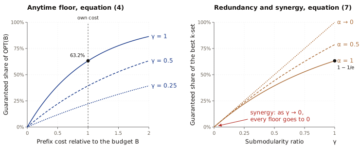
With diminishing returns the densities never rise, so the chain traces a concave curve of value against cost. Each prefix then satisfies an anytime bound against every budget B,9 where γ is the submodularity ratio10 (γ=1 under diminishing returns).
f(Sk)≥(1−e−γc(Sk)/B)OPT(B)
At its own cost, each prefix holds at least 1−1/e≈63.2% of the optimum.3 Unless P=NP, no polynomial-time rule guarantees more for maximum coverage.11 The bound is tight: a classical instance with geometrically shrinking rows runs along it.
Practice sits far above the floor. Across 80 random coverage instances computed for this construct, 93.4% of chain prefixes were exactly optimal at their own cost, and the worst held 87.9%.
When value is additive, the chain is exact at its breakpoints.12 Its prefixes are then the supported Pareto points, the maximizers of f(S)−λc(S) as λ falls.13 With overlap, the chain is the nested approximation of a frontier whose exact members reshuffle.
A fixed budget can strand one expensive, valuable input between breakpoints. Returning the better of the chain and the best single input restores half of 1−1/e.14
Compounding the other way: prerequisites
Item-by-item greedy fails when value comes in prerequisite chains. A foundation scores low on its own, so cheap self-contained inputs keep beating it. An advanced input scores near zero until its foundations land, so its full value never shows in advance.
The fix scores bundles instead of items. For each unread input e, take its prerequisite closure cl(e): e plus every unread input it depends on. Score the bundle on the residual, then commit it in prerequisite order.
ρ(e∣S)=c(cl(e)∖S)Δ(cl(e)∖S∣S)
A foundation now borrows the value of what it unlocks, so fundamentals move forward without hand-set importance weights. The exact rule scores every prerequisite-closed set of unread inputs; single closures are its practical approximation.
For additive value this is a solved problem in scheduling.15 Sidney’s decomposition (1975)16 repeatedly takes the prerequisite-closed set with the highest ratio of weight to processing time, and some optimal schedule respects it. Orders consistent with it keep value-weighted waiting time within a factor of 2 of optimal.171819
With overlap and prerequisites together, no clean constant is established.20 Closure density is the natural combination of the two solved cases: the residual from Section 4, the bundles from Sidney.
A worked example makes the trade concrete. Seven books cover eight concept areas weighted by importance, 28 points in total: math 4, neurons 3, networks 4, coding 4, plasticity 3, synthesis 5, methods 3, history 2.
Book
Pages
Teaches
Needs first
Overview survey
100
Neurons, networks, coding at survey depth
Nothing
Math primer
500
Math tools
Nothing
Canonical textbook
600
Neurons, networks, coding in depth
Math primer
Advanced synthesis
300
Synthesis
Canonical textbook
Plasticity monograph
200
Plasticity
Canonical textbook
Methods handbook
300
Methods
Nothing
History of the field
200
History
Nothing
Table 2. The seven-book shelf. Pages are the cost, the eight weighted concept areas are the value, and the last column is the prerequisite order.
A survey gives 30% mastery of what it touches and needs no foundations. A deep text gives full mastery with its foundations in place, and only 20% without them.
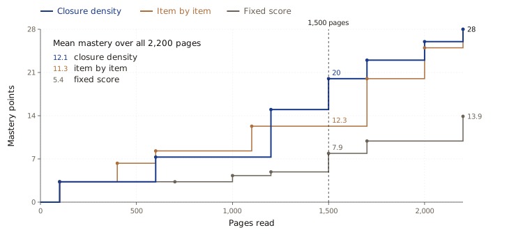
Figure 2. By 1,500 pages, closure density holds 20 of 28 mastery points. Mastery after each finished book on the shelf of Table 2, under three orderings: closure density (blue), item-by-item greedy (ochre) and the fixed impact-per-page score (grey). At 1,500 pages item by item holds 12.3 and the fixed score 7.9. The inset gives each ordering’s mean mastery over all 2,200 pages. Computed for this paper; code in Appendix A.
Item by item reads the quick, self-contained books first and leads until 1,100 pages. Closure density pays for the foundation first and overtakes at 1,200. Averaged over all 2,200 pages it holds 12.1 points at any moment, against 11.3 item by item and 5.4 for the fixed score.
The fixed score finishes the shelf with only 13.9 points. It reads the canonical textbook before the math primer, so the textbook’s depth never lands.
The stop: the shadow price of attention
The chain stops when the best density falls below λ, the value one unit of effort earns elsewhere. Stopping there maximizes value minus priced effort along the chain.
S(λ)=SK,K=max{k:ρk≥λ}=argkmax[f(Sk)−λc(Sk)]
λ is the Lagrange multiplier of the budget. The rule is the equimarginal principle:21 spend where marginal value per unit cost is highest, until it meets the price. Because densities never rise under diminishing returns, stops are nested: a higher price only truncates the same chain.
Reading has its own literature for this rule. Information foraging theory22 models a reader as a forager maximizing information gained per unit of time. Two of its results carry over directly.
The diet model. Admit sources in order of profitability, value per unit of handling time, while profitability exceeds the overall rate earned from the better sources alone.
The patch model. Charnov’s marginal value theorem (1976):23 leave a patch once its instantaneous rate of gain falls to the long-run average.
λ is therefore not a free parameter. It is the long-run rate of mastery per word, and the ordering itself determines it.
The true units are chapters, not books. A book is a patch with diminishing returns inside, so leave it once its marginal rate falls below λ.
Regimes and limits
Two measurable parameters set how far the chain can be trusted. Curvature α measures redundancy, from 0 for independent inputs to 1 for full overlap.24 The submodularity ratio γ measures synergy, from 1 for none down toward 0.
f(Sk)≥α1−e−αγ∣S∣≤kmaxf(S)
This bound holds under a cardinality constraint.25 Redundancy costs at most a factor of 1−1/e. Synergy has no floor: when inputs pay off only jointly, as in an exclusive-or pair, each looks worthless alone and the chain never starts.
Figure 3. Redundancy costs at most a factor of 1 − 1/e; synergy has no floor. Left: the anytime floor of equation (4), the share of OPT(B) a prefix is guaranteed, against the prefix’s cost relative to the budget, for submodularity ratios γ of 1, 0.5 and 0.25; at its own cost and with γ = 1 the floor is 63.2%. Right: the bound of equation (7) against γ for curvature α near 0, 0.5 and 1; at γ = 1 these give 100%, 78.7% and 63.2%, and every curve falls to zero as γ does. Analytic result; no data.
Each remaining limit has a known patch.
Synergy outside declared prerequisites. Bundle the complements into one composite input before running the chain, which restores γ.
A hard budget. Return the better of the budget-feasible chain and the best single input, or seed the chain with every set of three inputs to recover 1−1/e.26
A stream with irrevocable decisions. Replace the argmax with a density threshold. A grid of thresholds run in parallel guarantees 1/2−ε under a cardinality constraint, the best a small-memory single pass can do.2728
Value revealed only by reading. Use expected gain under the current belief; the adaptive chain keeps 1−1/e against the best adaptive policy.29
Friction. Words absorb faster once foundations are known, so cost depends on the state: c(e∣S). Re-scoring already uses the current cost, though the guarantees above assume fixed costs.
Scale. Gains only shrink, so a max-heap of stale gains needs re-scoring only at its top.30
One case stays open. Overlap and prerequisites together, under general costs, have no clean worst-case constant in the results gathered here.
Procedure
The construct runs in six steps, for a reading list or for any pool of inputs.
Inventory the value. List the concept areas the field requires, weighted by importance. For a system, list its needs, failure modes or open questions instead.
Map prerequisites. Record which concepts require which. Most fields have a short spine of foundations.
Map coverage. For each input, at chapter level, estimate how deeply it covers each concept. A table of contents or an LLM judge gives a usable first pass.
Price each input. Cost is words or hours, raised where the reader lacks the background.
Run the closure-density chain. Score each unread chapter together with its unread prerequisites, commit the best bundle, re-score, repeat.
Stop at λ. Set λ to your recent rate of mastery per hour; skip any chapter, or leave any book, whose density falls below it.
Revise as you go. Coverage estimates sharpen with each chapter read, which is the adaptive case of Section 8.
The answer
The greediest Pareto set has a precise name: the residual-density ordering, scored over prerequisite-closed bundles and stopped at the shadow price.
Key insight. As a policy for the shelf: read next whatever adds the most not-yet-known value per word, counting what it unlocks, and stop when that rate falls below your average.
Label. Residual-density ordering.
Line. Shadow-priced, prerequisite-closed residual-density ordering under diminishing returns, with per-prefix near-optimal value per unit effort.
Sentence. A nested selection sequence that commits, at each step, the prerequisite-closed bundle of maximal net-new value per unit cost, re-scored against the residual of every prior commit, and halts at the shadow price of effort.
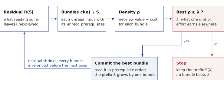
Figure 4. The policy loop: read the densest prerequisite-closed bundle next, until its density falls below λ. Each pass bundles every unread input with its unread prerequisites, scores each bundle’s net-new value per unit cost against the residual, and compares the best density with the shadow price λ. If it clears λ, the bundle is committed in prerequisite order and the loop runs again; if not, the loop stops and keeps the prefix S(λ). Conceptual schematic.
The loop runs until no bundle beats λ. Each commit shrinks the residual, which re-prices every remaining bundle before the next comparison: that feedback is the compounding the question asked for.
The seven-book example
The listing reproduces the numbers in Section 6 and Figures 1 and 2: the three orderings, mastery after each finished book, the mean over all 2,200 pages, and the best set within a budget. Mastery is exact (fractions), and ties in density go to the book listed first in Table 2.
from fractions import Fraction
from itertools import combinations
WEIGHTS = {'math': 4, 'neurons': 3, 'networks': 4, 'coding': 4,
'plasticity': 3, 'synthesis': 5, 'methods': 3, 'history': 2}
CORE = ('neurons', 'networks', 'coding')
# Table 2, in order: pages, concepts taught, the book that must come first.
BOOKS = {
'Overview survey': (100, CORE, None),
'Math primer': (500, ('math',), None),
'Canonical textbook': (600, CORE, 'Math primer'),
'Advanced synthesis': (300, ('synthesis',), 'Canonical textbook'),
'Plasticity monograph': (200, ('plasticity',), 'Canonical textbook'),
'Methods handbook': (300, ('methods',), None),
'History of the field': (200, ('history',), None),
}
SURVEY, UNPREPARED = Fraction(3, 10), Fraction(1, 5)
defmastery(order):
"""Mastery points after reading the books in `order`, in that order."""
depth, landed = {}, set()
for book in order:
_, concepts, needs = BOOKS[book]
if book == 'Overview survey':
level = SURVEY
elif needs isNoneor needs in landed:
level = 1
landed.add(book)
else:
level = UNPREPARED
for concept in concepts:
depth[concept] = max(depth.get(concept, 0), level)
returnsum(WEIGHTS[concept] * level for concept, level in depth.items())
defpages(books):
returnsum(BOOKS[book][0] for book in books)
defclosure(book, read):
"""`book` and every unread book it depends on, foundations first."""
bundle = []
while book isnotNoneand book notin read:
bundle.insert(0, book)
book = BOOKS[book][2]
return bundle
defgreedy(bundle_of):
"""Commit the bundle with the most net-new mastery per page; re-score; repeat."""
read = []
whilelen(read) < len(BOOKS):
bundles = [bundle_of(book, read) for book in BOOKS if book notin read]
read += max(bundles, key=lambda b: (mastery(read + b) - mastery(read)) / pages(b))
return read
defimpact_per_page(book):
"""The fixed score: full value per page, as if every foundation were in place."""
size, concepts, _ = BOOKS[book]
return Fraction(sum(WEIGHTS[concept] for concept in concepts), size)
ORDERS = {
'Closure density': greedy(closure),
'Item by item': greedy(lambda book, read: [book]),
'Fixed score': sorted(BOOKS, key=impact_per_page, reverse=True),
}
deftrajectory(order):
"""(pages read, mastery) after each finished book."""return [(pages(order[:k]), mastery(order[:k])) for k inrange(1, len(order) + 1)]
defheld_at(order, at):
"""Mastery held once `at` pages have been read."""returnmax([m for p, m in trajectory(order) if p <= at], default=0)
defaverage(order):
"""Mastery held at a moment chosen uniformly over the whole shelf's pages."""
steps = trajectory(order)
area = sum(m * (later - p) for (p, m), (later, _) inzip(steps, steps[1:]))
return area / pages(BOOKS)
# Every set, scored in Table 2 order, which already puts each foundation first.
SETS = [s for k inrange(len(BOOKS) + 1) for s in combinations(BOOKS, k)]
defbest(budget):
"""The exact frontier: the most mastery any set reaches within `budget` pages."""returnmax((mastery(s), s) for s in SETS if pages(s) <= budget)
for name, order in ORDERS.items():
held = ', '.join(f'{float(v):g}'for _, v in trajectory(order))
print(f'{name}: {held}; mean {float(average(order)):.1f}')
for budget in (600, 1100):
value, books = best(budget)
print(f'best within {budget:,} pages: {float(value):g}, {", ".join(books)}')
Output:
Closure density: 3.3, 7.3, 15, 20, 23, 26, 28; mean 12.1
Item by item: 3.3, 6.3, 8.3, 12.3, 20, 25, 28; mean 11.3
Fixed score: 3.3, 3.3, 4.3, 4.9, 7.9, 9.9, 13.9; mean 5.4
best within 600 pages: 8.3, Overview survey, Methods handbook, History of the field
best within 1,100 pages: 15, Math primer, Canonical textbook
The shelf behind the question
Book
Core foundation it contributes
Dayan & Abbott, Theoretical Neuroscience (2001)
Neural encoding and decoding, information in spike trains, conductance and network models
Izhikevich, Dynamical Systems in Neuroscience (2007)
Excitability as nonlinear dynamics: phase planes, limit cycles, bifurcations
Churchland & Sejnowski, The Computational Brain (1992)
The philosophy of neural computation
Strang, Introduction to Linear Algebra (2016)
Eigendecomposition, SVD, projections
Bear, Connors & Paradiso, Neuroscience: Exploring the Brain (2015)
Neuroanatomy and neurochemistry
Griffiths, Introduction to Electrodynamics (2017)
Field potentials, EEG forward models, cable theory
Leschziner, The Nocturnal Brain (2019)
Sleep–wake circuits and their disorders
Table 3. The shelf behind Section 1, from the original reading note: each book and the core foundation it contributes. The order is the note’s own ranking, which predates this paper and was not computed with the procedure of Section 9. Ten lighter titles on the note (popular science, sleep, learning workflow) are left out.
References
Footnotes
Streeter, M., & Golovin, D. (2008). An online algorithm for maximizing submodular functions. Advances in Neural Information Processing Systems, 21. proceedings.nips.cc. ↩
Nemhauser, G. L., Wolsey, L. A., & Fisher, M. L. (1978). An analysis of approximations for maximizing submodular set functions, I. Mathematical Programming, 14(1), 265–294. doi:10.1007/BF01588971. ↩↩2
Santos, R. L. T., Macdonald, C., & Ounis, I. (2010). Exploiting query reformulations for web search result diversification. In Proceedings of the 19th International Conference on World Wide Web (pp. 881–890). doi:10.1145/1772690.1772780. ↩
Chen, S., Billings, S. A., & Luo, W. (1989). Orthogonal least squares methods and their application to non-linear system identification. International Journal of Control, 50(5), 1873–1896. doi:10.1080/00207178908953472. ↩
Krause, A., & Guestrin, C. (2005). Near-optimal nonmyopic value of information in graphical models. In Proceedings of the 21st Conference on Uncertainty in Artificial Intelligence (UAI). arXiv:1207.1394. ↩
Kulesza, A., & Taskar, B. (2012). Determinantal point processes for machine learning. Foundations and Trends in Machine Learning, 5(2–3), 123–286. doi:10.1561/2200000044. ↩
Carbonell, J., & Goldstein, J. (1998). The use of MMR, diversity-based reranking for reordering documents and producing summaries. In Proceedings of the 21st Annual International ACM SIGIR Conference on Research and Development in Information Retrieval (pp. 335–336). doi:10.1145/290941.291025. ↩
Krause, A., & Golovin, D. (2014). Submodular function maximization. In L. Bordeaux, Y. Hamadi, & P. Kohli (Eds.), Tractability: Practical Approaches to Hard Problems (pp. 71–104). Cambridge University Press. doi:10.1017/CBO9781139177801.004. ↩
Das, A., & Kempe, D. (2018). Approximate submodularity and its applications: subset selection, sparse approximation and dictionary selection. Journal of Machine Learning Research, 19(3), 1–34. jmlr.org. Extends Das and Kempe (2011), Submodular meets spectral, ICML. ↩
Feige, U. (1998). A threshold of ln n for approximating set cover. Journal of the ACM, 45(4), 634–652. doi:10.1145/285055.285059. ↩
Dantzig, G. B. (1957). Discrete-variable extremum problems. Operations Research, 5(2), 266–288. doi:10.1287/opre.5.2.266. ↩
Ehrgott, M. (2005). Multicriteria optimization (2nd ed.). Springer. ↩
Khuller, S., Moss, A., & Naor, J. (1999). The budgeted maximum coverage problem. Information Processing Letters, 70(1), 39–45. doi:10.1016/S0020-0190(99)00031-9. The guarantee is conservative: Tang et al. (2021) show the same rule reaches at least 0.405 of the optimum, doi:10.1145/3447386. ↩
Smith, W. E. (1956). Various optimizers for single-stage production. Naval Research Logistics Quarterly, 3(1–2), 59–66. doi:10.1002/nav.3800030106. ↩
Sidney, J. B. (1975). Decomposition algorithms for single-machine sequencing with precedence relations and deferral costs. Operations Research, 23(2), 283–298. doi:10.1287/opre.23.2.283. ↩
Chekuri, C., & Motwani, R. (1999). Precedence constrained scheduling to minimize sum of weighted completion times on a single machine. Discrete Applied Mathematics, 98(1–2), 29–38. doi:10.1016/S0166-218X(98)00143-7. ↩
Margot, F., Queyranne, M., & Wang, Y. (2003). Decompositions, network flows, and a precedence constrained single-machine scheduling problem. Operations Research, 51(6), 981–992. doi:10.1287/opre.51.6.981.24912. ↩
Correa, J. R., & Schulz, A. S. (2005). Single-machine scheduling with precedence constraints. Mathematics of Operations Research, 30(4), 1005–1021. doi:10.1287/moor.1050.0158. Shows that virtually all known 2-approximations are consistent with Sidney’s decomposition. ↩
Tschiatschek, S., Singla, A., & Krause, A. (2017). Selecting sequences of items via submodular maximization. In Proceedings of the AAAI Conference on Artificial Intelligence, 31(1). doi:10.1609/aaai.v31i1.10923. Guarantees for a related case, value that depends on the order of items along a directed graph. ↩
Gossen, H. H. (1854). Entwickelung der Gesetze des menschlichen Verkehrs. Vieweg. ↩
Charnov, E. L. (1976). Optimal foraging, the marginal value theorem. Theoretical Population Biology, 9(2), 129–136. doi:10.1016/0040-5809(76)90040-X. ↩
Conforti, M., & Cornuéjols, G. (1984). Submodular set functions, matroids and the greedy algorithm: tight worst-case bounds and some generalizations of the Rado–Edmonds theorem. Discrete Applied Mathematics, 7(3), 251–274. doi:10.1016/0166-218X(84)90003-9. ↩
Bian, A. A., Buhmann, J. M., Krause, A., & Tschiatschek, S. (2017). Guarantees for greedy maximization of non-submodular functions with applications. In Proceedings of the 34th International Conference on Machine Learning, PMLR 70, 498–507. proceedings.mlr.press. ↩
Sviridenko, M. (2004). A note on maximizing a submodular set function subject to a knapsack constraint. Operations Research Letters, 32(1), 41–43. doi:10.1016/S0167-6377(03)00062-2. ↩
Badanidiyuru, A., Mirzasoleiman, B., Karbasi, A., & Krause, A. (2014). Streaming submodular maximization: massive data summarization on the fly. In Proceedings of the 20th ACM SIGKDD International Conference on Knowledge Discovery and Data Mining (pp. 671–680). doi:10.1145/2623330.2623637. ↩
Feldman, M., Norouzi-Fard, A., Svensson, O., & Zenklusen, R. (2023). The one-way communication complexity of submodular maximization with applications to streaming and robustness. Journal of the ACM, 70(4), 1–52. doi:10.1145/3588564. ↩
Golovin, D., & Krause, A. (2011). Adaptive submodularity: theory and applications in active learning and stochastic optimization. Journal of Artificial Intelligence Research, 42, 427–486. jair.org. ↩
Minoux, M. (1978). Accelerated greedy algorithms for maximizing submodular set functions. In Optimization Techniques, Lecture Notes in Control and Information Sciences, vol. 7 (pp. 234–243). Springer. doi:10.1007/BFb0006528. ↩
Cite as: Vicente González B.. “How should an overwhelming pool be sequenced so that every prefix holds the most net-new value per unit of effort?.” vicente.md/2026-004, 17 Oct 2026.← Archive